Fiber Optic Splitter Selection Guide: PLC vs FBT, Ratios & Connectors
By Jergeo Engineering Team | Published July 2026 · 9 min read

A fiber optic splitter divides one optical signal into multiple outputs. It is the core passive component in any PON (Passive Optical Network) — from FTTH last-mile deployments to campus distribution architectures. Choosing the wrong splitter means exceeding your optical power budget, which translates to signal drops, customer complaints, and costly rework.
Summary
PLC splitters are the standard for FTTH PON networks with split ratios of 1x16 and above, offering uniform power distribution across all outputs and full-band wavelength support from 1260 to 1650nm.
This guide covers how splitters work, the technical differences between PLC and FBT technologies, how to select split ratios, and how connector types and form factors affect your deployment. Where relevant, we reference specific Jergeo splitter models to ground the discussion in real hardware specs.
How fiber optic splitters work
A fiber optic splitter takes optical power from one input fiber and distributes it across multiple output fibers. The splitting is passive — no electrical power, no active components. Two technologies dominate the market: PLC (Planar Lightwave Circuit) and FBT (Fused Biconical Taper). Both achieve the same basic function but through different physical mechanisms, and they differ significantly in performance characteristics.
The key parameter is the split ratio, expressed as 1×N (one input, N outputs) or 2×N (two inputs, N outputs). A 1×8 splitter divides the input power among 8 output ports. In an ideal splitter with no excess loss, each output receives 1/N of the input power. The theoretical splitting loss for each ratio is calculated as 10×log₁₀(N) dB:
- 1×4: ~6.0 dB splitting loss
- 1×8: ~9.0 dB splitting loss
- 1×16: ~12.0 dB splitting loss
- 1×32: ~15.0 dB splitting loss
- 2×32: ~15.0 dB splitting loss (same per-port loss, but with a second input port for redundancy or dual-feed architectures)
Real-world insertion loss is always higher than the theoretical splitting loss due to excess loss from the splitting mechanism itself, connector losses, and splice losses. A typical 1×8 PLC splitter will show 10.5–11.5 dB total insertion loss per channel (including the ~9.0 dB splitting loss plus ~1.5–2.5 dB excess loss). The exact number depends on the manufacturer's process quality and the connector polish type.
PLC splitters vs FBT splitters: what actually differs
The two splitter technologies are not interchangeable in most modern deployments. Here is what you need to know:
FBT splitters work by fusing and tapering two or more fibers together until their cores are close enough for optical power to transfer between them. This process is repeated in stages to achieve higher split ratios. FBT is a mature technology that has been used for decades. It handles uneven split ratios well — you can get a 1×2 splitter with a 90:10 ratio, which is useful for monitoring taps.
PLC splitters use a silica glass chip with waveguides etched into it using lithography. The input waveguide branches into N output waveguides through a Y-junction cascade on the chip. The result is much tighter uniformity across all output ports — typically within ±1.5 dB for a 1×32 PLC splitter, compared to potentially ±3–4 dB variation in a cascaded FBT design.
| Parameter | PLC Splitter | FBT Splitter |
|---|---|---|
| Splitting mechanism | Planar waveguide chip | Fused & tapered fibers |
| Max split ratio | 1×64 (standard) | 1×32 (practical limit) |
| Port uniformity (1×32) | ±1.5 dB typical | ±3–4 dB (cascaded) |
| Wavelength range | 1260–1650 nm (full band) | 1260–1650 nm, but ±2 dB variation across band |
| Operating temperature | -40 to +85°C | -40 to +85°C (standard); degrades at extremes |
| Custom split ratios | Fixed (equal split only) | Flexible (e.g. 90:10, 80:20) |
| Physical size | Compact for high split ratios | Larger for equivalent high-ratio splits |
| Cost at 1×4 or 1×8 | Moderate | Lower for low-ratio splits |
| Best application | FTTH PON, high-density ODN | Small-split monitoring, legacy networks |
For any FTTH or PON deployment with split ratios of 1×16 or higher, PLC splitters are the standard choice. FBT splitters remain useful when you need an uneven split (for example, a 95:5 tap for inline optical power monitoring) or a simple 1×2 or 1×4 split at the lowest cost point.
Split ratio selection: matching the network design
The split ratio is the single most impactful decision in ODN design. It determines how many subscribers share one OLT PON port, and it sets the insertion loss budget for the entire optical link. Here is the practical decision framework:
1×4 splitters — Used in small MDU (Multi-Dwelling Unit) deployments or early-stage FTTH networks where subscriber density is low. The 6.0 dB splitting loss leaves maximum headroom for long feeder cables. You can cascade two 1×4 splitters to reach 16 subscribers, but at the cost of an additional splitting stage and its associated loss.
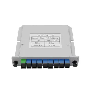
1×8 splitters — The most common ratio in urban FTTH deployments. The Jergeo JPLCC-8A is a card-type 1×8 PLC splitter in a 130×110×25 mm form factor with SC or LC adapters (PC/UPC/APC polish available). Its card-type form factor slots into standard splitter panels and ODFs, making it the workhorse unit for wall-mount or rack-mount distribution boxes serving 4–8 subscribers per splitter.
1×16 splitters — Used when subscriber density supports 16 endpoints per PON port, or in secondary splitting stages where a 1×8 primary splitter feeds into a 1×2 secondary. The Jergeo JPLCT-16A is a tray-type chassis (300×180×25 mm) with FC, SC, or LC adapter options. Its tray form factor fits standard 19" rack enclosures and provides organized cable management for 16 output ports.
1×32 splitters — The maximum single-stage split for GPON/EPON deployments. At ~15 dB splitting loss plus excess loss, a 1×32 configuration pushes the limits of standard Class B+ OLT optics (which budget ~28 dB total link loss). The Jergeo JPLCT-32A is a tray-type chassis (310×180×51 mm) supporting FC, SC, or LC adapters with PC/UPC/APC polish. The 51 mm height accommodates the fiber routing and splice trays needed for 32 output ports.
2×32 splitters — Adds a second input port for redundancy or dual-feed architectures (e.g., RF video overlay alongside data). Both input ports connect to 32 output ports. Used in networks where service continuity matters and a backup OLT PON port is required.
Budget planning: insertion loss by split ratio
Insertion loss budgeting is where theoretical design meets field reality. Every component in the optical path adds loss. The table below shows typical values for planning purposes:
| Split Ratio | Theoretical Split Loss | Typical Excess Loss | Total Insertion Loss (typical) |
|---|---|---|---|
| 1×4 | 6.0 dB | ~1.0–1.5 dB | 7.0–8.0 dB |
| 1×8 | 9.0 dB | ~1.5–2.0 dB | 10.5–11.5 dB |
| 1×16 | 12.0 dB | ~2.0–2.5 dB | 14.0–15.0 dB |
| 1×32 | 15.0 dB | ~2.5–3.0 dB | 17.5–18.5 dB |
| 2×32 | 15.0 dB | ~2.5–3.0 dB | 17.5–18.5 dB |
These values are per splitter. In a cascaded architecture (e.g., 1×4 + 1×8), you add the insertion loss of both stages. A two-stage split of 1×4 followed by 1×8 gives you 32 endpoints but at a total splitter loss of ~25–29 dB — which may exceed the optical power budget of Class B+ GPON optics (28 dB budget). Always run the full link budget calculation: OLT transmit power minus receiver sensitivity must exceed the sum of fiber attenuation (dB/km), connector losses (0.2–0.5 dB per connection), splice losses (0.05–0.1 dB per splice), and splitter insertion loss.
Connector types and polish options
Connectors on a fiber optic splitter determine how it interfaces with the rest of the ODN. Three connector types are standard:
- SC connectors — 2.5 mm ferrule, push-pull coupling. Most common in FTTH deployments worldwide. Available in both UPC and APC polish.
- LC connectors — 1.25 mm ferrule, latch-type coupling. Higher density than SC. Common in data center and enterprise ODN environments where panel port density matters.
- FC connectors — 2.5 mm ferrule, screw-on coupling. Higher mechanical retention than SC. Used in environments with vibration (industrial, outdoor cabinet deployments).
The polish type matters more than many installers realize:
- UPC (Ultra Physical Contact) — Return loss ≥50 dB. Blue color coding on the adapter/boot. Standard for data and most GPON deployments.
- APC (Angled Physical Contact) — Return loss ≥60 dB. Green color coding. Required for RF video overlay (CATV over PON) because the 8° angle prevents reflected light from interfering with analog video signals. Also specified in XGS-PON and NG-PON2 deployments where higher return loss improves signal integrity.
- PC (Physical Contact) — Return loss ≥35 dB. Legacy polish type, largely replaced by UPC in modern deployments.
All three Jergeo splitter models — JPLCC-8A, JPLCT-16A, and JPLCT-32A — support PC, UPC, and APC polish types across their available connector options. When specifying a fiber splitter SC APC configuration, make sure the matching patch cords and adapters also use APC polish — mixing UPC and APC in the same link causes ~0.5 dB additional loss and degrades return performance.
Form factors: cassette, card type, and tray type
The physical packaging of the splitter determines how it integrates into your distribution infrastructure. Three form factors are common:
Bare fiber (pigtail) splitters — No connectors, no housing. Just the splitting element with bare fiber pigtails for field splicing. Lowest cost, smallest size. Used inside closure joints and splice trays where space is constrained. Requires fusion splicing on every port.
Card type splitters — Mounted on a rigid card (typically ABS plastic) with adapter ports on the front. The Jergeo JPLCC-8A (130×110×25 mm) is a typical card type design. It slides into a standard splitter slot in fiber distribution boxes and ODFs. The card protects the fragile splitting element and provides strain relief for the fiber pigtails. Card type units are the most common format for street cabinets and wall-mount enclosures.
Tray type / chassis splitters — Larger housings designed for 19" rack mounting. The Jergeo JPLCT-16A (300×180×25 mm, 1×16) and Jergeo JPLCT-32A (310×180×51 mm, 1×32) are tray type designs. They integrate splice management, fiber routing channels, and adapter panels into a single unit. Tray type splitters are the preferred format for central offices and high-density distribution points where organized cable management and port labeling matter.
Fiber optic splitter cassettes — Modular plug-and-play units that combine a splitter with an enclosure and pre-terminated connectors. Cassettes plug into a standard adapter panel (like a fiber distribution box) and can be swapped without disturbing other splitter channels. They trade some density for faster installation and easier maintenance.
Selecting the right form factor for your deployment
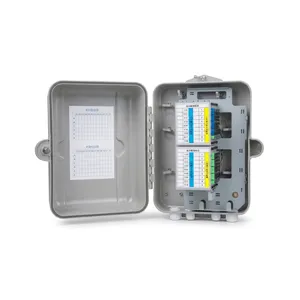
- FTTH drop point (wall-mount box, 4–8 subscribers): Card type splitter (e.g., JPLCC-8A) inside a small distribution box. Low cost, compact, fast to deploy.
- FTTH secondary distribution (street cabinet, 16 subscribers): Tray type splitter (e.g., JPLCT-16A) in a floor-standing or pole-mount cabinet. Provides organized port management for field technicians.
- Central office / headend (32+ subscribers per PON): Tray type splitter (e.g., JPLCT-32A) in a 19" rack or ODF. Highest port density, best cable management, supports future reconfiguration.
- Rapid deployment or temporary sites: Fiber optic splitter cassette in a plug-and-play distribution box. Pre-terminated, no field splicing required.
Environmental and reliability considerations
All Jergeo PLC splitter models (JPLCC-8A, JPLCT-16A, JPLCT-32A) are rated for -40 to +85°C operating temperature. This covers outdoor cabinet deployments in most climate zones. For splitter installations in direct sunlight or desert environments, ensure the cabinet itself provides adequate thermal management — the splitter spec assumes the fiber reaches thermal equilibrium within the housing, not that the housing absorbs full solar loading.
PLC splitters are inherently more reliable than FBT in high-split-ratio applications because the waveguide chip is a single monolithic component. FBT splitters at 1×16 or 1×32 are actually cascades of multiple 1×2 splitting stages, each of which is a potential failure point. A single bad fusion joint in a cascaded FBT splitter can take out an entire branch — whereas a PLC chip failure typically affects all ports equally (and rarely occurs outside of physical damage).
Related Products
References
- ITU-T G.671 — transmission characteristics of passive optical components including splitters
- FOA Splitter Guide — The Fiber Optic Association reference on passive optical splitters
Key takeaway
For any PON deployment at 1×16 or higher, specify PLC splitters — the uniformity, wavelength flatness, and temperature stability outperform FBT at these ratios. Match the split ratio to your OLT optical power budget: 1×8 for Class B+ GPON with long feeder runs, 1×16 for balanced urban deployments, and 1×32 only when fiber count and subscriber density justify the tighter loss budget. Choose card type for drop points and tray type for central offices. Always match connector polish types end-to-end (APC to APC, UPC to UPC) — mixing them adds loss and kills return performance.
Related products
Related Articles
FTTH Network Architecture Guide
Understand the full ODN hierarchy from OLT to ONT — and where splitters fit in the signal path.
Read Article →
ODN Equipment Complete Guide
Complete list of all passive fiber network components and their roles in the ODN.
Read Article →
Fiber Distribution Cabinet Buying Guide
How to spec the right FDC with built-in splitter module slots for your FTTH deployment.
Read Article →